EO tutorial¶

This notebook demonstrates python programming applied to Earth Observation, within the VRE with the following tools :

• Jupyter notebook
• Python, numpy, matplotlib
• EODAG
• Xarray
• Rasterio
• Folium
• QGISLab

This tutorial is inspired by a research article by M. Urban et. al. that you can download from this link

During the southern summer season of 2015 and 2016, South Africa experienced one of the most severe meteorological droughts since the start of climate recording, due to an exceptionally strong El Niño event. To investigate spatiotemporal dynamics of surface moisture and vegetation structure, data from ESA’s Copernicus Sentinel-1/-2 and NASA’s Landsat-8 for the period between March 2015 and November 2017 were utilized

In the research article, several techniques and indices were computed to assess the severity of the drought and their temporal variations.

Here, we will limit the study to the computation of the vegetation index to compare vegetation status between dry (April to October) and wet (November to April) seasons, both visually and numerically.

The NDWI will also be used to visualise variation in water level.

Import all the modules needed for the exercise¶

First, we load the lab_black extension that will format the code cells properly

In [1]:

%load_ext lab_black

%load_ext lab_black

Then, let's import all the required modules

In [2]:

import os

import xarray  # Data storage/format
import rasterio  # Image manipulation
from rasterio.plot import show  # display images
import numpy as np  # Mathematical python module
from IPython.display import Markdown  # Nicer display
import folium  # Display
from eodag import EODataAccessGateway  # Query data catalog
from qgislab import qgislab  # Display
from ipyleaflet import Map, basemaps, LayersControl  # Display

import os import xarray # Data storage/format import rasterio # Image manipulation from rasterio.plot import show # display images import numpy as np # Mathematical python module from IPython.display import Markdown # Nicer display import folium # Display from eodag import EODataAccessGateway # Query data catalog from qgislab import qgislab # Display from ipyleaflet import Map, basemaps, LayersControl # Display

Fetch the products with EODAG¶

Two Sentinel products were pre-selected to show the most difference between dry and wet seasons

Execute the cell below to get the products: all the available products are stored in the object "search_results", a list of EO_products (see EODAG documentation for more details)

In [3]:

Injected by EODAG plugin

dag = EODataAccessGateway()
product_type = "S2_MSI_L1C"
footprint = {"lonmin": 31, "latmin": -26, "lonmax": 32, "latmax": -25}
cloud_cover = 4
start, end = "2016-08-31", "2017-02-01"
search_results, estimated_total_nbr_of_results = dag.search(
    productType=product_type,
    box=footprint,
    start=start,
    end=end,
    cloudCover=cloud_cover,
)

dag = EODataAccessGateway() product_type = "S2_MSI_L1C" footprint = {"lonmin": 31, "latmin": -26, "lonmax": 32, "latmax": -25} cloud_cover = 4 start, end = "2016-08-31", "2017-02-01" search_results, estimated_total_nbr_of_results = dag.search( productType=product_type, box=footprint, start=start, end=end, cloudCover=cloud_cover, )

'box' or 'bbox' parameters are only supported for backwards  compatibility reasons. Usage of 'geom' is recommended.

All available tiles found with the parameters above can be located on a map

In [4]:

emap = folium.Map([-25, 31], zoom_start=7)
layer = folium.features.GeoJson(
    data=search_results.as_geojson_object(),
    tooltip=folium.GeoJsonTooltip(fields=["title"]),
).add_to(emap)
emap

emap = folium.Map([-25, 31], zoom_start=7) layer = folium.features.GeoJson( data=search_results.as_geojson_object(), tooltip=folium.GeoJsonTooltip(fields=["title"]), ).add_to(emap) emap

Out[4]:

Make this Notebook Trusted to load map: File -> Trust Notebook

The name of the two products to download for the demo is given below

In [5]:

# Search results by name
title_wet = (
    "S2A_MSIL1C_20170119T074231_N0204_R092_T36JUT_20170119T075734"  # January 2017
)
title_dry = (
    "S2A_MSIL1C_20160901T073612_N0204_R092_T36JUT_20160901T080536"  # September 2016
)

# Search results by name title_wet = ( "S2A_MSIL1C_20170119T074231_N0204_R092_T36JUT_20170119T075734" # January 2017 ) title_dry = ( "S2A_MSIL1C_20160901T073612_N0204_R092_T36JUT_20160901T080536" # September 2016 )

To retrieve these two products only, we need to find the indices of the products corresponding to the titles above. We will also print the cloud cover to make sure it is 0%

In [6]:

for i, p in enumerate(search_results):
    if p.properties["title"] == title_wet or p.properties["title"] == title_dry:
        display(
            Markdown(
                (
                    "Cloud cover: {0} - ID: *{1}* - **Index: {2}**".format(
                        p.properties["cloudCover"], p.properties["id"], i
                    )
                )
            )
        )

for i, p in enumerate(search_results): if p.properties["title"] == title_wet or p.properties["title"] == title_dry: display( Markdown( ( "Cloud cover: {0} - ID: *{1}* - **Index: {2}**".format( p.properties["cloudCover"], p.properties["id"], i ) ) ) )

Cloud cover: 0 - ID: S2A_MSIL1C_20170119T074231_N0204_R092_T36JUT_20170119T075734 - Index: 5

Cloud cover: 0 - ID: S2A_MSIL1C_20160901T073612_N0204_R092_T36JUT_20160901T080536 - Index: 17

EODAG search results properties are stored in the form of a dictionnary that you can access via .properties

These properties inlude the name of the instrument, the platform, dates, title, description of the bands, etc.

In [7]:

# Print list of properties
search_results[0].properties

# Print list of properties search_results[0].properties

Out[7]:

{'abstract': None,
 'instrument': 'MSI',
 'platform': 'S2ST',
 'platformSerialIdentifier': 'S2A',
 'processingLevel': 'LEVEL1C',
 'sensorType': 'OPTICAL',
 'license': 'proprietary',
 'missionStartDate': '2015-06-23T00:00:00Z',
 'title': 'S2A_MSIL1C_20170119T074231_N0204_R092_T36JTS_20170119T075734',
 'bands': [{'name': 'B01',
   'common_name': 'coastal',
   'center_wavelength': 0.4439,
   'full_width_half_max': 0.027,
   'gsd': 60},
  {'name': 'B02',
   'common_name': 'blue',
   'center_wavelength': 0.4966,
   'full_width_half_max': 0.098,
   'gsd': 10},
  {'name': 'B03',
   'common_name': 'green',
   'center_wavelength': 0.56,
   'full_width_half_max': 0.045,
   'gsd': 10},
  {'name': 'B04',
   'common_name': 'red',
   'center_wavelength': 0.6645,
   'full_width_half_max': 0.038,
   'gsd': 10},
  {'name': 'B05',
   'center_wavelength': 0.7039,
   'full_width_half_max': 0.019,
   'gsd': 20},
  {'name': 'B06',
   'center_wavelength': 0.7402,
   'full_width_half_max': 0.018,
   'gsd': 20},
  {'name': 'B07',
   'center_wavelength': 0.7825,
   'full_width_half_max': 0.028,
   'gsd': 20},
  {'name': 'B08',
   'common_name': 'nir',
   'center_wavelength': 0.8351,
   'full_width_half_max': 0.145,
   'gsd': 10},
  {'name': 'B8A',
   'center_wavelength': 0.8648,
   'full_width_half_max': 0.033,
   'gsd': 20},
  {'name': 'B09',
   'center_wavelength': 0.945,
   'full_width_half_max': 0.026,
   'gsd': 60},
  {'name': 'B10',
   'common_name': 'cirrus',
   'center_wavelength': 0.13735,
   'full_width_half_max': 0.075,
   'gsd': 60},
  {'name': 'B11',
   'common_name': 'swir16',
   'center_wavelength': 0.16137,
   'full_width_half_max': 0.075,
   'gsd': 20},
  {'name': 'B12',
   'common_name': 'swir22',
   'center_wavelength': 0.22024,
   'full_width_half_max': 0.242,
   'gsd': 20}],
 'productType': 'S2MSI1C',
 'uid': '029637ca-98ec-5e3e-b6be-00aee47a0009',
 'keyword': {'b1f9871e461ff4c': {'name': 'Africa',
   'normalized': 'africa',
   'type': 'continent',
   'href': 'https://peps.cnes.fr/resto/api/collections/S2ST/search.json?&lang=en&q=Africa'},
  '4df8db701d09747': {'name': 'South Africa',
   'normalized': 'south-africa',
   'type': 'country',
   'parentHash': 'b1f9871e461ff4c',
   'value': 97.24,
   'href': 'https://peps.cnes.fr/resto/api/collections/S2ST/search.json?&lang=en&q=%22South%20Africa%22'},
  'da0fbc17ed3f64d': {'name': '_all',
   'normalized': '_all',
   'type': 'region',
   'parentHash': '4df8db701d09747',
   'href': 'https://peps.cnes.fr/resto/api/collections/S2ST/search.json?&lang=en&q=_all'},
  '5be5a17052913a8': {'name': 'Mpumalanga',
   'normalized': 'mpumalanga',
   'type': 'state',
   'parentHash': 'da0fbc17ed3f64d',
   'value': 97.24,
   'href': 'https://peps.cnes.fr/resto/api/collections/S2ST/search.json?&lang=en&q=Mpumalanga'},
  'f91f7d4bbcee9de': {'name': 'Swaziland',
   'normalized': 'swaziland',
   'type': 'country',
   'parentHash': 'b1f9871e461ff4c',
   'value': 2.72,
   'href': 'https://peps.cnes.fr/resto/api/collections/S2ST/search.json?&lang=en&q=Swaziland'},
  'f70cb7d971c9f09': {'name': '_all',
   'normalized': '_all',
   'type': 'region',
   'parentHash': 'f91f7d4bbcee9de',
   'href': 'https://peps.cnes.fr/resto/api/collections/S2ST/search.json?&lang=en&q=_all'},
  '19729bf2ea55752': {'name': 'Hhohho',
   'normalized': 'hhohho',
   'type': 'state',
   'parentHash': 'f70cb7d971c9f09',
   'value': 2.72,
   'href': 'https://peps.cnes.fr/resto/api/collections/S2ST/search.json?&lang=en&q=Hhohho'},
  'd817ecd5e7765d3': {'name': 'Southern',
   'type': 'location',
   'href': 'https://peps.cnes.fr/resto/api/collections/S2ST/search.json?&lang=en&q=Southern'},
  '6278eea013ff0d3': {'name': 'Summer',
   'type': 'season',
   'href': 'https://peps.cnes.fr/resto/api/collections/S2ST/search.json?&lang=en&q=Summer'},
  '45038f3c2322ea3': {'name': 'S2ST',
   'type': 'collection',
   'href': 'https://peps.cnes.fr/resto/api/collections/S2ST/search.json?&lang=en&q=S2ST'},
  '6219554ecf5905c': {'name': 'S2MSI1C',
   'type': 'productType',
   'href': 'https://peps.cnes.fr/resto/api/collections/S2ST/search.json?&lang=en&q=S2MSI1C'},
  '44b15c0a6e62129': {'name': 'LEVEL1C',
   'type': 'processingLevel',
   'href': 'https://peps.cnes.fr/resto/api/collections/S2ST/search.json?&lang=en&q=LEVEL1C'},
  'afe9ad14455c260': {'name': 's2A',
   'type': 'platform',
   'href': 'https://peps.cnes.fr/resto/api/collections/S2ST/search.json?&lang=en&q=s2A'},
  '503f8f6199f3e44': {'name': 'msi',
   'type': 'instrument',
   'parentHash': 'afe9ad14455c260',
   'href': 'https://peps.cnes.fr/resto/api/collections/S2ST/search.json?&lang=en&q=msi'},
  '3f85bb5d775e1fc': {'name': 'INS-NOBS',
   'type': 'sensorMode',
   'parentHash': '503f8f6199f3e44',
   'href': 'https://peps.cnes.fr/resto/api/collections/S2ST/search.json?&lang=en&q=INS-NOBS'},
  'e8f96b7c46c0d54': {'name': 'Descending',
   'type': 'orbitDirection',
   'href': 'https://peps.cnes.fr/resto/api/collections/S2ST/search.json?&lang=en&q=Descending'},
  'c0706bb19e22342': {'name': '0',
   'type': 'isNrt',
   'href': 'https://peps.cnes.fr/resto/api/collections/S2ST/search.json?&lang=en&q=0'},
  'adbd1cc9d2fe94b': {'name': 'Nominal',
   'type': 'realtime',
   'parentHash': 'c0706bb19e22342',
   'href': 'https://peps.cnes.fr/resto/api/collections/S2ST/search.json?&lang=en&q=Nominal'},
  'f48375ec19410fc': {'name': '2017',
   'type': 'year',
   'href': 'https://peps.cnes.fr/resto/api/collections/S2ST/search.json?&lang=en&q=2017'},
  'de07f3fd5ed39a8': {'name': 'January',
   'type': 'month',
   'parentHash': 'f48375ec19410fc',
   'href': 'https://peps.cnes.fr/resto/api/collections/S2ST/search.json?&lang=en&q=January'},
  '451a5e6ed3d50de': {'name': '19',
   'type': 'day',
   'parentHash': 'de07f3fd5ed39a8',
   'href': 'https://peps.cnes.fr/resto/api/collections/S2ST/search.json?&lang=en&q=19'}},
 'resolution': None,
 'organisationName': None,
 'publicationDate': '2017-02-04T03:15:22.349Z',
 'parentIdentifier': 'urn:ogc:def:EOP:ESA::SENTINEL-2:',
 'orbitNumber': 8240,
 'orbitDirection': 'descending',
 'cloudCover': 0,
 'snowCover': None,
 'creationDate': '2017-01-19T17:21:59.494Z',
 'modificationDate': '2017-02-04T03:15:22.349Z',
 'sensorMode': 'INS-NOBS',
 'startTimeFromAscendingNode': '2017-01-19T07:42:31.026Z',
 'completionTimeFromAscendingNode': '2017-01-19T07:42:31.026Z',
 'id': 'S2A_MSIL1C_20170119T074231_N0204_R092_T36JTS_20170119T075734',
 'quicklook': 'https://peps.cnes.fr/quicklook/2017/01/19/S2A/S2A_MSIL1C_20170119T074231_N0204_R092_T36JTS_20170119T075734_quicklook.jpg',
 'downloadLink': 'https://peps.cnes.fr/resto/collections/S2ST/029637ca-98ec-5e3e-b6be-00aee47a0009/download',
 'storageStatus': 'ONLINE',
 'thumbnail': None,
 'resourceSize': 763820014,
 'resourceChecksum': ' 3C43B9A9C2AB9E8F0FD834F84B3BDCE1',
 'visible': 1,
 'newVersion': None,
 'isNrt': 0,
 'realtime': 'Nominal',
 'relativeOrbitNumber': 92,
 's2TakeId': 'GS2A_20170119T074231_008240_N02.04',
 'mgrs': '36JTS',
 'bareSoil': None,
 'highProbaClouds': None,
 'mediumProbaClouds': None,
 'lowProbaClouds': None,
 'snowIce': None,
 'vegetation': None,
 'water': None,
 'services': {'browse': {'title': 'Display full resolution product on map',
   'layer': {'type': 'WMS',
    'url': 'https://peps.cnes.fr/cgi-bin/mapserver?map=WMS_S2ST&data=2017/01/19/S2A/S2A_MSIL1C_20170119T074231_N0204_R092_T36JTS_20170119T075734',
    'layers': ''}},
  'download': {'url': 'https://peps.cnes.fr/resto/collections/S2ST/029637ca-98ec-5e3e-b6be-00aee47a0009/download',
   'mimeType': 'application/zip',
   'size': 763820014,
   'checksum': ' 3C43B9A9C2AB9E8F0FD834F84B3BDCE1'}},
 'links': [{'rel': 'alternate',
   'type': 'application/json',
   'title': 'GeoJSON link for 029637ca-98ec-5e3e-b6be-00aee47a0009',
   'href': 'https://peps.cnes.fr/resto/collections/S2ST/029637ca-98ec-5e3e-b6be-00aee47a0009.json?&lang=en'},
  {'rel': 'alternate',
   'type': 'application/atom+xml',
   'title': 'ATOM link for 029637ca-98ec-5e3e-b6be-00aee47a0009',
   'href': 'https://peps.cnes.fr/resto/collections/S2ST/029637ca-98ec-5e3e-b6be-00aee47a0009.atom?&lang=en'}],
 'storage': {'mode': 'disk'}}

Now we know exactly which product to download, we can launch the download process

To simplify the work and limit bandwith usage, the products have been downloaded and stored on the local drive

The products have also already been croped to the same area as in the research article with QGIS.

Warning: The cell below is fully commented, do not execute it. It is here as a reference.

In [9]:

# Execute this cell only once !!!
# If executed by mistake cancel notebook execution
# products_to_download = [search_results[5], search_results[17]]
# paths = dag.download(products_to_download)

# Execute this cell only once !!! # If executed by mistake cancel notebook execution # products_to_download = [search_results[5], search_results[17]] # paths = dag.download(products_to_download)

Once the products are downloaded we can start our work

Quick display¶

We will start by displaying the product on an interactive map to locate the area that we will use in the exercise. To display the product properly, we will need to find the central coordinates of the product as well as those of its boundaries (top left corner & bottom right corner)

Open the True-Colour Image with rasterio

In [10]:

src_tci_img = rasterio.open("Dry_season/TCI_epsg4326.tif")

src_tci_img = rasterio.open("Dry_season/TCI_epsg4326.tif")

Now, get the bounds of the tiff files

In [11]:

x1_tci, y1_tci, x2_tci, y2_tci = src_tci_img.bounds  # Get coordinates of image bounds
Markdown(
    "**Bounds of the layer**<br />Bottom left: {0} {1}<br />Top right: {2} {3}".format(
        x1_tci, y1_tci, x2_tci, y2_tci
    )
)

x1_tci, y1_tci, x2_tci, y2_tci = src_tci_img.bounds # Get coordinates of image bounds Markdown( "**Bounds of the layer**
Bottom left: {0} {1}
Top right: {2} {3}".format( x1_tci, y1_tci, x2_tci, y2_tci ) )

Out[11]:

Bounds of the layer
Bottom left: 31.450673332 -25.043673318
Top right: 31.520626766 -24.994216109

To center the display, we also need the longitude and latitude of the product. Fortunatyle, rasterio can get these values with the method lnglat()

In [12]:

lon, lat = src_tci_img.lnglat()  # Get longitude and latitude
m = folium.Map(location=[lat, lon], zoom_start=12)

folium.raster_layers.ImageOverlay(
    image=src_tci_img.read()[0],
    bounds=[[y1_tci, x1_tci], [y2_tci, x2_tci]],
    opacity=0.7,
).add_to(m)

m

lon, lat = src_tci_img.lnglat() # Get longitude and latitude m = folium.Map(location=[lat, lon], zoom_start=12) folium.raster_layers.ImageOverlay( image=src_tci_img.read()[0], bounds=[[y1_tci, x1_tci], [y2_tci, x2_tci]], opacity=0.7, ).add_to(m) m

Out[12]:

Make this Notebook Trusted to load map: File -> Trust Notebook

The work area is located East of South Africa

Read data¶

The first step consists in opening all the required data.

The data is stored on the drive, one file for each band, that we will open one by one

Open files¶

Using xarray & rasterio, we will open the following bands for both WET and DRY regions :

• B03 (green)
• B04 (red)
• NIR (B08)
• NIR_A (B08A)
• SWIR (B11)

Data is stored into two separate Xarrays (one for each season).

In [13]:

# January 2017 - Wet season
base_path_wet = "Wet_season/"
# blue_wet = xarray.open_rasterio(os.path.join(base_path_wet, "B02.tif"))
green_wet = xarray.open_rasterio(
    os.path.join(base_path_wet, "B03_epsg4326.tif")
)  # 554x698
red_wet = xarray.open_rasterio(
    os.path.join(base_path_wet, "B04_epsg4326.tif")
)  # 554x698
nir_wet = xarray.open_rasterio(
    os.path.join(base_path_wet, "B08_epsg4326.tif")
)  # 554x698
nir_A_wet = xarray.open_rasterio(
    os.path.join(base_path_wet, "B08A_epsg4326.tif")
)  # 277x349
swir_wet = xarray.open_rasterio(
    os.path.join(base_path_wet, "B11_epsg4326.tif")
)  # 277x349

# Septembre 2016 - Dry saison
base_path_dry = "Dry_season/"
# blue_dry = xarray.open_rasterio(os.path.join(base_path, "B02.tif"))
green_dry = xarray.open_rasterio(os.path.join(base_path_dry, "B03_epsg4326.tif"))
red_dry = xarray.open_rasterio(os.path.join(base_path_dry, "B04_epsg4326.tif"))
nir_dry = xarray.open_rasterio(os.path.join(base_path_dry, "B08_epsg4326.tif"))
nir_A_dry = xarray.open_rasterio(
    os.path.join(base_path_dry, "B08A_epsg4326.tif")
)  # 277x349
swir_dry = xarray.open_rasterio(
    os.path.join(base_path_dry, "B11_epsg4326.tif")
)  # 277x349

# January 2017 - Wet season base_path_wet = "Wet_season/" # blue_wet = xarray.open_rasterio(os.path.join(base_path_wet, "B02.tif")) green_wet = xarray.open_rasterio( os.path.join(base_path_wet, "B03_epsg4326.tif") ) # 554x698 red_wet = xarray.open_rasterio( os.path.join(base_path_wet, "B04_epsg4326.tif") ) # 554x698 nir_wet = xarray.open_rasterio( os.path.join(base_path_wet, "B08_epsg4326.tif") ) # 554x698 nir_A_wet = xarray.open_rasterio( os.path.join(base_path_wet, "B08A_epsg4326.tif") ) # 277x349 swir_wet = xarray.open_rasterio( os.path.join(base_path_wet, "B11_epsg4326.tif") ) # 277x349 # Septembre 2016 - Dry saison base_path_dry = "Dry_season/" # blue_dry = xarray.open_rasterio(os.path.join(base_path, "B02.tif")) green_dry = xarray.open_rasterio(os.path.join(base_path_dry, "B03_epsg4326.tif")) red_dry = xarray.open_rasterio(os.path.join(base_path_dry, "B04_epsg4326.tif")) nir_dry = xarray.open_rasterio(os.path.join(base_path_dry, "B08_epsg4326.tif")) nir_A_dry = xarray.open_rasterio( os.path.join(base_path_dry, "B08A_epsg4326.tif") ) # 277x349 swir_dry = xarray.open_rasterio( os.path.join(base_path_dry, "B11_epsg4326.tif") ) # 277x349

Print the products sizes to make sure they are correctly opened

In [14]:

display(Markdown("Red Band dimensions: {0}".format(red_wet.shape)))
display(Markdown("NIR Band dimensions: {0}".format(nir_wet.shape)))
display(Markdown("Green Band dimensions: {0}".format(green_wet.shape)))
display(Markdown("NIR-A Band dimensions: {0}".format(nir_A_wet.shape)))
display(Markdown("SWIR Band dimensions: {0}".format(swir_wet.shape)))
display(Markdown("Red Band dimensions: {0}".format(red_dry.shape)))
display(Markdown("NIR Band dimensions: {0}".format(nir_dry.shape)))
display(Markdown("Green Band dimensions {0}:".format(green_dry.shape)))
display(Markdown("NIR-A Band dimensions {0}:".format(nir_A_dry.shape)))
display(Markdown("SWIR Band dimensions {0}:".format(swir_dry.shape)))

display(Markdown("Red Band dimensions: {0}".format(red_wet.shape))) display(Markdown("NIR Band dimensions: {0}".format(nir_wet.shape))) display(Markdown("Green Band dimensions: {0}".format(green_wet.shape))) display(Markdown("NIR-A Band dimensions: {0}".format(nir_A_wet.shape))) display(Markdown("SWIR Band dimensions: {0}".format(swir_wet.shape))) display(Markdown("Red Band dimensions: {0}".format(red_dry.shape))) display(Markdown("NIR Band dimensions: {0}".format(nir_dry.shape))) display(Markdown("Green Band dimensions {0}:".format(green_dry.shape))) display(Markdown("NIR-A Band dimensions {0}:".format(nir_A_dry.shape))) display(Markdown("SWIR Band dimensions {0}:".format(swir_dry.shape)))

Red Band dimensions: (1, 554, 698)

NIR Band dimensions: (1, 554, 698)

Green Band dimensions: (1, 554, 698)

NIR-A Band dimensions: (1, 277, 349)

SWIR Band dimensions: (1, 277, 349)

Red Band dimensions: (1, 554, 698)

NIR Band dimensions: (1, 554, 698)

Green Band dimensions (1, 554, 698):

NIR-A Band dimensions (1, 277, 349):

SWIR Band dimensions (1, 277, 349):

Create Data Arrays¶

In this section we will create Data Arrays containing all the products opened above to perform computations

In [15]:

red_dry

red_dry

Out[15]:

<xarray.DataArray (band: 1, y: 554, x: 698)>
[386692 values with dtype=uint16]
Coordinates:
  * band     (band) int64 1
  * y        (y) float64 -24.99 -24.99 -24.99 -24.99 ... -25.04 -25.04 -25.04
  * x        (x) float64 31.45 31.45 31.45 31.45 ... 31.52 31.52 31.52 31.52
Attributes:
    transform:      (0.00010021981948423859, 0.0, 31.450673332, 0.0, -8.92729...
    crs:            +init=epsg:4326
    res:            (0.00010021981948423859, 8.92729404332127e-05)
    is_tiled:       0
    nodatavals:     (0.0,)
    scales:         (1.0,)
    offsets:        (0.0,)
    AREA_OR_POINT:  Area

Note that the coordinate 'Band' has no particular name, so we will need to name each band for all Data Arrays

For each band xarray, rename the band name to an understandable one:

e.g. red['band'] = ['red']

In [16]:

# Affect correct name to bands in the data array
red_dry["band"] = ["red"]
green_dry["band"] = ["green"]
# blue_dry["band"] = ["blue"]
nir_dry["band"] = ["nir"]
nir_A_dry["band"] = ["nir_a"]
swir_dry["band"] = ["swir"]
red_wet["band"] = ["red"]
green_wet["band"] = ["green"]
# blue_wet["band"] = ["blue"]
nir_wet["band"] = ["nir"]
nir_A_wet["band"] = ["nir_a"]
swir_wet["band"] = ["swir"]

# Affect correct name to bands in the data array red_dry["band"] = ["red"] green_dry["band"] = ["green"] # blue_dry["band"] = ["blue"] nir_dry["band"] = ["nir"] nir_A_dry["band"] = ["nir_a"] swir_dry["band"] = ["swir"] red_wet["band"] = ["red"] green_wet["band"] = ["green"] # blue_wet["band"] = ["blue"] nir_wet["band"] = ["nir"] nir_A_wet["band"] = ["nir_a"] swir_wet["band"] = ["swir"]

Display the same DataArray as above to check its band has been correctly renamed

In [17]:

display(Markdown(str(red_dry.coords)))

display(Markdown(str(red_dry.coords)))

Coordinates:

• band (band) <U3 'red'
• y (y) float64 -24.99 -24.99 -24.99 -24.99 ... -25.04 -25.04 -25.04
• x (x) float64 31.45 31.45 31.45 31.45 ... 31.52 31.52 31.52 31.52

In the following steps we will compute both NDVI and NDWI.

Note that NDWI uses band B08A and B11 (or B12) while NDVI bands B03 and B08. These bands do not have the same shape : 277x349 vs 554x698, so we can not merge these bands into the same DataArray easily.

This difference in shape is due to the resolution of these bands

Since not all bands yield the same resolution, we will separate the data and therefore concatenate the data into Xarrays :

• One for Red, NIR, Green bands
• One for NIR-A & SWIR bands

Now, create the 4 data arrays (two per season) by concatenating the required bands

In [18]:

da_wet_a = xarray.concat([red_wet, green_wet, nir_wet], dim="band")  # For NDVI
da_wet_b = xarray.concat([nir_A_wet, swir_wet], dim="band")  # For NDWI
da_dry_a = xarray.concat([red_dry, green_dry, nir_dry], dim="band")  # For NDVI
da_dry_b = xarray.concat([nir_A_dry, swir_dry], dim="band")  # For NDWI

da_wet_a = xarray.concat([red_wet, green_wet, nir_wet], dim="band") # For NDVI da_wet_b = xarray.concat([nir_A_wet, swir_wet], dim="band") # For NDWI da_dry_a = xarray.concat([red_dry, green_dry, nir_dry], dim="band") # For NDVI da_dry_b = xarray.concat([nir_A_dry, swir_dry], dim="band") # For NDWI

Clean both data arrays by replacing N/A values by zero

In [19]:

da_wet_a = da_wet_a.fillna(0)
da_wet_b = da_wet_b.fillna(0)
da_dry_a = da_dry_a.fillna(0)
da_dry_b = da_dry_b.fillna(0)

da_wet_a = da_wet_a.fillna(0) da_wet_b = da_wet_b.fillna(0) da_dry_a = da_dry_a.fillna(0) da_dry_b = da_dry_b.fillna(0)

Computations¶

Let's compute NDVI and NDWI

Compute the NDVI¶

Remember that:

$$ \text{NDVI} = \frac{Red - NIR}{Red + NIR} $$

Where Red is the red band (B03) and NIR the Near Infrared one (B08)

Do not forget to replace N/A values by zero

In [20]:

NDVI_wet = (da_wet_a.sel(band="nir") - da_wet_a.sel(band="red")) / (
    da_wet_a.sel(band="nir") + da_wet_a.sel(band="red")
)
NDVI_wet = NDVI_wet.fillna(0)  # Clean NDVI data by replacing N/A by 0

NDVI_wet = (da_wet_a.sel(band="nir") - da_wet_a.sel(band="red")) / ( da_wet_a.sel(band="nir") + da_wet_a.sel(band="red") ) NDVI_wet = NDVI_wet.fillna(0) # Clean NDVI data by replacing N/A by 0

In [21]:

NDVI_dry = (da_dry_a.sel(band="nir") - da_dry_a.sel(band="red")) / (
    da_dry_a.sel(band="nir") + da_dry_a.sel(band="red")
)
NDVI_dry = NDVI_dry.fillna(0)  # Clean NDVI data by replacing N/A by 0

NDVI_dry = (da_dry_a.sel(band="nir") - da_dry_a.sel(band="red")) / ( da_dry_a.sel(band="nir") + da_dry_a.sel(band="red") ) NDVI_dry = NDVI_dry.fillna(0) # Clean NDVI data by replacing N/A by 0

Let's print the maximum and minimum values of the NDVI for both seasons

In [22]:

max_wet = np.float(max(NDVI_wet[0]))
min_wet = np.float(min(NDVI_wet[0]))
max_dry = np.float(max(NDVI_dry[0]))
min_dry = np.float(min(NDVI_dry[0]))
display(Markdown("Maximum NDVI for **WET** season = {:.2f}".format(max_wet)))
display(Markdown("Maximum NDVI for **DRY** season = {:.2f}".format(max_dry)))
display(Markdown("The NDVI is much lower during the dry season"))

max_wet = np.float(max(NDVI_wet[0])) min_wet = np.float(min(NDVI_wet[0])) max_dry = np.float(max(NDVI_dry[0])) min_dry = np.float(min(NDVI_dry[0])) display(Markdown("Maximum NDVI for **WET** season = {:.2f}".format(max_wet))) display(Markdown("Maximum NDVI for **DRY** season = {:.2f}".format(max_dry))) display(Markdown("The NDVI is much lower during the dry season"))

Maximum NDVI for WET season = 0.69

Maximum NDVI for DRY season = 0.18

The NDVI is much lower during the dry season

We can perform a quick check of these computations of the NDVI by displaying it with the built-in plot() method

Since we plot a vegetation index, we'll select the "Greens" colormap.

The levels are indexed to the minimum and maximum values of the NDVI computed for the wet season

See matplotlib's documentation for more informations

In [23]:

plot = NDVI_wet.plot(
    levels=np.arange(min_wet, max_wet, 0.01), cmap="Greens"
)  # We assign the plotting function to a variable to avoid useless information display

plot = NDVI_wet.plot( levels=np.arange(min_wet, max_wet, 0.01), cmap="Greens" ) # We assign the plotting function to a variable to avoid useless information display

In [24]:

plot = NDVI_dry.plot(
    levels=np.arange(min_wet, max_wet, 0.01), cmap="Greens"
)  # We assign the plotting function to a variable to avoid useless information display

plot = NDVI_dry.plot( levels=np.arange(min_wet, max_wet, 0.01), cmap="Greens" ) # We assign the plotting function to a variable to avoid useless information display

Notice the variation in vegetation index depending on the season.

During the dry season, we can see that the vegetation has decreased except on the river's border

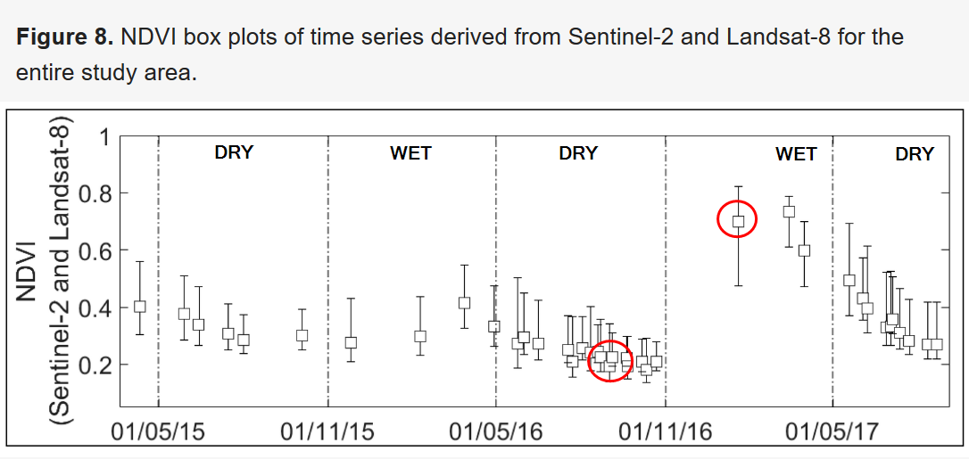
Note that these results are in good agreement with those observed in the article by Urban et. al. as shown in the graph below. The periods corresponding to our products are circled in red.

Evaluate the average vegetation¶

We can also use Xarray built-in mean() method to compute the mean value of the NDVI for both seasons.

In [25]:

display(
    Markdown(
        "The average NDVI for the wet season is: **{:.2f}**".format(
            np.float(NDVI_wet.mean())
        )
    )
)
display(
    Markdown(
        "The average NDVI for the dry season is: **{:.2f}**".format(
            np.float(NDVI_dry.mean())
        )
    )
)

display( Markdown( "The average NDVI for the wet season is: **{:.2f}**".format( np.float(NDVI_wet.mean()) ) ) ) display( Markdown( "The average NDVI for the dry season is: **{:.2f}**".format( np.float(NDVI_dry.mean()) ) ) )

The average NDVI for the wet season is: 0.59

The average NDVI for the dry season is: 0.15

Compute the NDWI¶

We can also compute the NDWI, using the following formula

$$ \text{NDWI} = \frac{(NIR - SWIR)}{NIR + SWIR} $$

Where NIR is band B08A and SWIR band B11

In [26]:

NDWI_wet = (da_wet_b.sel(band="nir_a") - da_wet_b.sel(band="swir")) / (
    da_wet_b.sel(band="nir_a") + da_wet_b.sel(band="swir")
)
NDWI_wet = NDWI_wet.fillna(0)

NDWI_wet = (da_wet_b.sel(band="nir_a") - da_wet_b.sel(band="swir")) / ( da_wet_b.sel(band="nir_a") + da_wet_b.sel(band="swir") ) NDWI_wet = NDWI_wet.fillna(0)

Plot the computed NDWI indices for both seasons and compare the results visually

In [27]:

NDWI_dry = (da_dry_b.sel(band="nir_a") - da_dry_b.sel(band="swir")) / (
    da_dry_b.sel(band="nir_a") + da_dry_b.sel(band="swir")
)
NDWI_dry = NDWI_dry.fillna(0)

NDWI_dry = (da_dry_b.sel(band="nir_a") - da_dry_b.sel(band="swir")) / ( da_dry_b.sel(band="nir_a") + da_dry_b.sel(band="swir") ) NDWI_dry = NDWI_dry.fillna(0)

In [28]:

plot = NDWI_wet.plot(
    levels=np.arange(0, 25, 0.1), cmap="Blues"
)  # We assign the plotting function to a variable to avoid useless information display

plot = NDWI_wet.plot( levels=np.arange(0, 25, 0.1), cmap="Blues" ) # We assign the plotting function to a variable to avoid useless information display

In [29]:

plot = NDWI_dry.plot(
    levels=np.arange(10, 35, 1), cmap="Blues"
)  # We assign the plotting function to a variable to avoid useless information display

plot = NDWI_dry.plot( levels=np.arange(10, 35, 1), cmap="Blues" ) # We assign the plotting function to a variable to avoid useless information display

Interactive plots¶

Export the computed NDVI to local files¶

To display the data into interactive plots, we have to:

• fetch the width and height of the products by opening a reference image: i.e. any of the original products with rasterio
• export the data to display as .tif files with rasterio
• use QGISLab to export these products to Cloud Optimised Gifs (COG)

In [30]:

src_img = rasterio.open("Dry_season/B03_epsg4326.tif")
width = src_img.width
height = src_img.height
display(
    Markdown(
        ("Image dimensions:\nwidth **{0}px** - height **{1}px**".format(width, height))
    )
)

src_img = rasterio.open("Dry_season/B03_epsg4326.tif") width = src_img.width height = src_img.height display( Markdown( ("Image dimensions:\nwidth **{0}px** - height **{1}px**".format(width, height)) ) )

Image dimensions: width 698px - height 554px

Now write the NDVI for wet and dry seasons

In [31]:

def write_file(src_img, data, outname):
    ndviImage = rasterio.open(
        outname,
        "w",
        driver="Gtiff",
        width=src_img.width,
        height=src_img.height,
        count=1,  # number of bands (1 for NDVI)
        crs=src_img.crs,
        transform=src_img.transform,
        dtype="float64",
    )
    ndviImage.write(data, 1)
    ndviImage.close()  # Do not forget to close opened file !


write_file(src_img, NDVI_wet, "NDVI_wet.tif")
write_file(src_img, NDVI_dry, "NDVI_dry.tif")

def write_file(src_img, data, outname): ndviImage = rasterio.open( outname, "w", driver="Gtiff", width=src_img.width, height=src_img.height, count=1, # number of bands (1 for NDVI) crs=src_img.crs, transform=src_img.transform, dtype="float64", ) ndviImage.write(data, 1) ndviImage.close() # Do not forget to close opened file ! write_file(src_img, NDVI_wet, "NDVI_wet.tif") write_file(src_img, NDVI_dry, "NDVI_dry.tif")

Open and display the written NDVI files to make sure they were properly written

In [32]:

ndvi_dry_src = rasterio.open("NDVI_dry.tif")
ndvi_wet_src = rasterio.open("NDVI_wet.tif")
show(ndvi_dry_src, cmap="Greens", title="NDVI for DRY SEASON")
show(ndvi_wet_src, cmap="Greens", title="NDVI for WET SEASON")

ndvi_dry_src = rasterio.open("NDVI_dry.tif") ndvi_wet_src = rasterio.open("NDVI_wet.tif") show(ndvi_dry_src, cmap="Greens", title="NDVI for DRY SEASON") show(ndvi_wet_src, cmap="Greens", title="NDVI for WET SEASON")

Out[32]:

<AxesSubplot:title={'center':'NDVI for WET SEASON'}>

Display the NDVI on an interactive map¶

Use QGISLab to convert both NDVI data to COG

In [33]:

# NDVI (GeoTiff) to COG
output_NDVI_wet_cog = "NDVI_wet_cog"
qgislab.cogify(
    src_path="NDVI_wet.tif",
    dst_path=output_NDVI_wet_cog,
    profile="deflate",
    resampling="average",
    overview_resampling="average",
    web_optimized=True,
    add_mask=False,
    nodata=0,
)

output_NDVI_dry_cog = "NDVI_dry_cog"
qgislab.cogify(
    src_path="NDVI_dry.tif",
    dst_path=output_NDVI_dry_cog,
    profile="deflate",
    resampling="average",
    overview_resampling="average",
    web_optimized=True,
    add_mask=False,
    nodata=0,
)

# NDVI (GeoTiff) to COG output_NDVI_wet_cog = "NDVI_wet_cog" qgislab.cogify( src_path="NDVI_wet.tif", dst_path=output_NDVI_wet_cog, profile="deflate", resampling="average", overview_resampling="average", web_optimized=True, add_mask=False, nodata=0, ) output_NDVI_dry_cog = "NDVI_dry_cog" qgislab.cogify( src_path="NDVI_dry.tif", dst_path=output_NDVI_dry_cog, profile="deflate", resampling="average", overview_resampling="average", web_optimized=True, add_mask=False, nodata=0, )

Reading input: NDVI_wet.tif
Adding overviews...
Updating dataset tags...
Writing output to: NDVI_wet_cog
Reading input: NDVI_dry.tif
Adding overviews...
Updating dataset tags...
Writing output to: NDVI_dry_cog

You should now have two cog files on the local drive

Using QGISLab, create layers that will be superimposed on the map

In [34]:

# Create layers
NDVI_wet_cog_layer = qgislab.build_layer(
    datafile_path=str(output_NDVI_wet_cog),
    display_name="NDVI WET SEASON layer",
    style_file_path="QGIS_NDVI_style.qml",
)

NDVI_dry_cog_layer = qgislab.build_layer(
    datafile_path=str(output_NDVI_dry_cog),
    display_name="NDVI DRY SEASON layer",
    style_file_path="QGIS_NDVI_style.qml",
)

# Create layers NDVI_wet_cog_layer = qgislab.build_layer( datafile_path=str(output_NDVI_wet_cog), display_name="NDVI WET SEASON layer", style_file_path="QGIS_NDVI_style.qml", ) NDVI_dry_cog_layer = qgislab.build_layer( datafile_path=str(output_NDVI_dry_cog), display_name="NDVI DRY SEASON layer", style_file_path="QGIS_NDVI_style.qml", )

Finally display all layers on the map

In [35]:

# Display
# NDVI_file = rasterio.open("NDVI_image.tif")
# img_lon, img_lat = NDVI_file.lnglat()
m = Map(basemap=basemaps.CartoDB.Positron, center=(lat, lon), zoom=12)

m.add_layer(NDVI_wet_cog_layer)
m.add_layer(NDVI_dry_cog_layer)

control = LayersControl(position="topright")
m.add_control(control)
m

# Display # NDVI_file = rasterio.open("NDVI_image.tif") # img_lon, img_lat = NDVI_file.lnglat() m = Map(basemap=basemaps.CartoDB.Positron, center=(lat, lon), zoom=12) m.add_layer(NDVI_wet_cog_layer) m.add_layer(NDVI_dry_cog_layer) control = LayersControl(position="topright") m.add_control(control) m

Map(center=[-25.018944713499998, 31.485650049], controls=(ZoomControl(options=['position', 'zoom_in_text', 'zo…

You can click on the top right "layers" icon to select which layer to display

Extra work : code optimisation¶

In this section we will demonstrate how Numba can help speed up computations

To do so, we will compute several vegation indices using different formulae

"Excess Green minus Excess Red" (ExGR) as proposed by Neto et. al.

Though less accurate than NDVI, ExGR (and similar) is useful when the NIR band is not available.

The formula is given below :

$$ \text{ExGR} = \frac{3G-2.4R-B}{R+G+B} $$

Where R, G, B correspond to bands Red, Green, Blue respectively

The Enhanced Vegetation Index (EVI2) that is less sensitive than NDVI to biophysical quantities such as vegetation fraction or leaf area index and whose use is therefore weakened with increasing vegetation densities beyond a threshold (see this article for example).

The EVI2 is :

$$ \text{EVI2} = 2.5 \times \frac{NIR - R}{NIR + (6 - 7.5/2.08)\times R +1} $$

Finally, we will compute the RDVI :

$$ \text{RDVI} = \frac{NIR - R}{\sqrt{(R + NIR)}} $$

Open files¶

For the sake of this demonstration, we will compute the indices with numpy instead of Xarray

Open all the band files needed to perform the computations using rasterio

In [36]:

blue_src = rasterio.open(os.path.join(base_path_wet, "B02_epsg4326.tif"))  # 554x698
green_src = rasterio.open(os.path.join(base_path_wet, "B03_epsg4326.tif"))  # 554x698
red_src = rasterio.open(os.path.join(base_path_wet, "B04_epsg4326.tif"))  # 554x698
nir_src = rasterio.open(os.path.join(base_path_wet, "B08_epsg4326.tif"))  # 554x698

blue = blue_src.read()
green = green_src.read()
red = red_src.read()
nir = nir_src.read()

blue_src = rasterio.open(os.path.join(base_path_wet, "B02_epsg4326.tif")) # 554x698 green_src = rasterio.open(os.path.join(base_path_wet, "B03_epsg4326.tif")) # 554x698 red_src = rasterio.open(os.path.join(base_path_wet, "B04_epsg4326.tif")) # 554x698 nir_src = rasterio.open(os.path.join(base_path_wet, "B08_epsg4326.tif")) # 554x698 blue = blue_src.read() green = green_src.read() red = red_src.read() nir = nir_src.read()

Computations¶

First, define a method that will compute the 4 different vegetation indices

In [37]:

np.seterr(divide="ignore", invalid="ignore")  # suppress warning


def compute_VI_np(blue, green, red, nir):
    """
    This method computes several vegetation indexes
    """
    EVI2 = 2.5 * (nir - red) / ((nir + (6 - 7.5 / 2.08) * red) + 1)
    NDVI = (nir - red) / (nir + red)
    RDVI = (nir - red) / np.sqrt(red + nir)
    ExGR = (3 * green - 2.4 * red - blue) / (red + green + blue)
    return EVI2, NDVI, RDVI, ExGR

np.seterr(divide="ignore", invalid="ignore") # suppress warning def compute_VI_np(blue, green, red, nir): """ This method computes several vegetation indexes """ EVI2 = 2.5 * (nir - red) / ((nir + (6 - 7.5 / 2.08) * red) + 1) NDVI = (nir - red) / (nir + red) RDVI = (nir - red) / np.sqrt(red + nir) ExGR = (3 * green - 2.4 * red - blue) / (red + green + blue) return EVI2, NDVI, RDVI, ExGR

Next, we write the same method, but use Numba to perform Just In Time compilation (we simply add a @jit decorator)

In [38]:

from numba import jit


@jit(nopython=True, parallel=True)
def compute_VI_numba(blue, green, red, nir):
    """
    This method computes several vegetation indexes
    """
    EVI2 = 2.5 * (nir - red) / ((nir + (6 - 7.5 / 2.08) * red) + 1)
    NDVI = (nir - red) / (nir + red)
    RDVI = (nir - red) / np.sqrt(red + nir)
    ExGR = (3 * green - 2.4 * red - blue) / (red + green + blue)
    return EVI2, NDVI, RDVI, ExGR

from numba import jit @jit(nopython=True, parallel=True) def compute_VI_numba(blue, green, red, nir): """ This method computes several vegetation indexes """ EVI2 = 2.5 * (nir - red) / ((nir + (6 - 7.5 / 2.08) * red) + 1) NDVI = (nir - red) / (nir + red) RDVI = (nir - red) / np.sqrt(red + nir) ExGR = (3 * green - 2.4 * red - blue) / (red + green + blue) return EVI2, NDVI, RDVI, ExGR

Evaluate the time needed to perform the computations with numpy only

In [39]:

%%timeit -r 5
EVI2, NDVI, RDVI, ExGR = compute_VI_np(blue, green, red, nir)

%%timeit -r 5 EVI2, NDVI, RDVI, ExGR = compute_VI_np(blue, green, red, nir)

10.9 ms ± 29.2 µs per loop (mean ± std. dev. of 5 runs, 100 loops each)

In [40]:

%%timeit -r 5
EVI2, NDVI, RDVI, ExGR = compute_VI_numba(blue, green, red, nir)

%%timeit -r 5 EVI2, NDVI, RDVI, ExGR = compute_VI_numba(blue, green, red, nir)

/usr/local/lib/python3.6/dist-packages/numba/np/ufunc/parallel.py:365: NumbaWarning: The TBB threading layer requires TBB version 2019.5 or later i.e., TBB_INTERFACE_VERSION >= 11005. Found TBB_INTERFACE_VERSION = 9107. The TBB threading layer is disabled.
  warnings.warn(problem)

4.1 ms ± 53.4 µs per loop (mean ± std. dev. of 5 runs, 1 loop each)

Notice that the computation time has been divided by more than 2

Display results¶

In [41]:

from matplotlib import pyplot as plt

EVI2, NDVI, RDVI, ExGR = compute_VI_numba(blue, green, red, nir)
formulas = ["EVI2", "NDVI", "RDVI", "ExGR"]
fig, axs = plt.subplots(nrows=2, ncols=2)
axs[0, 0].imshow(EVI2[0])
axs[0, 1].imshow(NDVI[0])
axs[1, 0].imshow(RDVI[0])
axs[1, 1].imshow(ExGR[0])
for i, ax in enumerate(axs.ravel()):  # ravel() reshapes the 2x2 dim array in a 1D array
    ax.set_title(formulas[i])
    ax.set_xticks([])  # Remove ticks from axes
    ax.set_yticks([])
plt.tight_layout()

from matplotlib import pyplot as plt EVI2, NDVI, RDVI, ExGR = compute_VI_numba(blue, green, red, nir) formulas = ["EVI2", "NDVI", "RDVI", "ExGR"] fig, axs = plt.subplots(nrows=2, ncols=2) axs[0, 0].imshow(EVI2[0]) axs[0, 1].imshow(NDVI[0]) axs[1, 0].imshow(RDVI[0]) axs[1, 1].imshow(ExGR[0]) for i, ax in enumerate(axs.ravel()): # ravel() reshapes the 2x2 dim array in a 1D array ax.set_title(formulas[i]) ax.set_xticks([]) # Remove ticks from axes ax.set_yticks([]) plt.tight_layout()